Implementing a MLP with numpy
Motivation
During my deep learning class of 2023, we were asked to build from a MLP with numpy. We trained the multilayer perceptron with the MNIST dataset.The goal was to develop a primitive but working implementation of a MLP with the help of Numpy. I won’t go over the exact details of the experimentation. The experimentation was originally coded in a colab notebook.
import matplotlib.pyplot as plt
import seaborn as sns
import numpy as np
import random
sns.set()

if __name__ == "__main__":
  # load data
  from tensorflow.keras.datasets import mnist
  (x_train, y_train), (x_test, y_test) = mnist.load_data()
Implementing a single Perceptron with NumPy
The perceptron function is defined as:
\[\begin{equation} f(x) = \begin{cases} 1 \text{ if } w \cdot x+b > 0 \\ 0 \text{ otherwise} \end{cases} \end{equation}\]In the section below, we are implementing a perceptron with the ReLu activation function and the absolute loss function.
class BinaryPerceptron:
  def __init__(self, input_dim):
    '''
    Initialize perceptron with random parameters
    '''
    self.w = np.random.randn(input_dim)
    self.b = 0

  def relu(self, x):
    '''
    Implement the ReLu function

    :param x: input tensor

    :return: x after ReLu function
    '''
    zeros = np.zeros_like(x)

    # return ...
    return np.maximum(x,zeros)

  def fire(self, x):
    '''
    function determining whether perceptron is activated/fired given stimulus x.
    (Corresponds to f(x) above)

    :param x: input tensor

    :return: 1 if perceptron is fired, 0 otherwise
    '''
    # o = ...
    o = np.dot(self.w,x)+self.b
    a = self.relu(o).item(0)
    return 1 if a > 0 else 0

  def train(self, x, y, lr):
    '''
    Manual implementation of the backpropagation algorithm

    :param x: input vector x
    :param y: target label y
    :param lr: learning rate

    :return: l1 loss
    '''
    y_hat = self.fire(x)
    diff = y - y_hat

    # gradient_w
    zeros = np.zeros_like(x)
    sgn = np.sign(diff)
    grad_w = -sgn*np.maximum(zeros, x)
    # gradienb_b
    grad_b = -sgn*np.ones_like(x)
    # update self.w
    self.w = self.w - lr* grad_w
    # update self.b
    self.b = self.b - lr* grad_b

    loss = np.abs(diff)
    return loss
The following section is devoted to training our new Perceptron on a synthethic binary classification dataset, using a learning rate of 0.001. The model is trained for 3 epochs.
if __name__ == "__main__":

  # Generate binary synthetic data and define graph function
  # 100 data points of class 0 centered at (-5, -5)
  # 100 data points of class 1 centered at (5, 5)
  num_samples = 100
  np.random.seed(42)
  X_class0 = np.random.randn(num_samples, 2) + np.array([-5, 5])
  np.random.seed(42)
  X_class1 = np.random.randn(num_samples, 2) + np.array([5, 5])
  X = np.vstack([X_class0, X_class1])
  y = np.hstack([np.zeros(num_samples), np.ones(num_samples)])
  np.random.seed(42)
  shuffle_idx = np.random.permutation(len(X))
  X = X[shuffle_idx]
  y = y[shuffle_idx]

  def graph(X, y, perceptron, title):
    plt.scatter(X[:, 0], X[:, 1], c=y, cmap=plt.cm.Paired, label="Data points")
    x_min, x_max = X[:, 0].min() - 1, X[:, 0].max() + 1
    y_min, y_max = X[:, 1].min() - 1, X[:, 1].max() + 1
    xx, yy = np.meshgrid(np.arange(x_min, x_max, 0.1),
                        np.arange(y_min, y_max, 0.1))
    Z = np.array([perceptron.fire(np.array([x, y])) for x, y in np.c_[xx.ravel(), yy.ravel()]])
    Z = Z.reshape(xx.shape)
    plt.contourf(xx, yy, Z, alpha=0.3, cmap=plt.cm.Paired, levels=[-1, 0, 1])
    plt.title(title)
    plt.show()

  # Train the perceptron
  num_epochs = 3
  perceptron = BinaryPerceptron(input_dim=2)
  for i in range(num_epochs):
    losses = []
    for j in range(num_samples * 2):
      print(perceptron.w)
      loss = perceptron.train(x = X[j], y = y[j], lr = 0.001)
      losses.append(loss)

    graph(X, y, perceptron, f'Perceptron Decision Boundary after epoch {i + 1}')
    print(f"    accuracy after epoch {i + 1}: ", sum(1 for loss in losses if loss == 0) / (num_samples * 2))
Here is the resulting decision boundary:
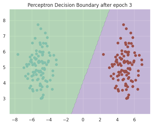
Our classifier was able to have 100% accuracy. In the real world, such results are unlikely as this training set was simple: it is linearly separable.
Implementing MLPs with NumPy
Multilayers perceptron are nothing more than a stack of Perceptrons. This simple idea allows to build much more complex decision boundary, thanks to the nonlinearity added by the activation function. The following code results in a ‘homemade’ numpy MLP.
\[\begin{aligned} \mathbf{o_{l+1}} &= \mathbf{W_l} \cdot \mathbf{a_l} + \mathbf{b_l} \\ \mathbf{a_{l+1}} &= \mathbf{a(o_{l+1})}, \end{aligned}\]where $\mathbf{o_{l+1}}$ is the preactivation output of the next layer, $\mathbf{a_{l+1}}$ is the output of the next layer. For the first/input layer, $\mathbf{a_l}$ is the input. For the last/output layer, we use the softmax activation function paired with cross-entropy loss.
import math
class MLP(object):

  def __init__(self,
               layer_dims = (784, 128, 64, 10),
               activation = "relu",
               epsilon = 1e-6,
               lr = 0.01
               ):
    super().__init__()

    assert activation in ["relu", "sigmoid", "tanh"], "activation function needs to be among relu, sigmoid, tanh."
    self.layer_dims = layer_dims
    self.activation = activation
    self.epsilon = epsilon
    self.lr = lr
    self.init_parameters()

  def init_parameters(self):
    '''
    Initialize model parameters

    '''
    self.parameters = []
    for i, layer_dim in enumerate(self.layer_dims[:-1]):
      #w_shape = (self.layer_dims[i+1], layer_dim)
      w_shape = (layer_dim , self.layer_dims[i+1] )
      w = np.random.uniform(-1/math.sqrt(self.layer_dims[0]),1/math.sqrt(self.layer_dims[0]),w_shape)
      # b =
      b = np.zeros((1,self.layer_dims[i+1]))
      self.parameters.append({f'w' : w, f'b' : b})

  def activation_fn(self, x):
    '''
    Implementation of relu, sigmoid and tanh activation functions

    :param x: input (preactivation) vector

    :return: input after activation function
    '''
    if self.activation == "relu":
      return np.maximum(0, x)
    elif self.activation == "sigmoid":
      return np.divide(np.ones_like(x) , (np.ones_like(x) + np.exp(-x)))
    elif self.activation == "tanh":
      return np.tanh(x)

  def gradient_activation_fn(self, x):
    '''
    Implementation of the derivative function of the relu, sigmoid and tanh activation functions

    :param x: input (postactivation) vector

    :return: input after derivative of activation function
    '''
    if self.activation == "relu":
      return np.where(x <= 0, 0, 1)

    elif self.activation == "sigmoid":
      return (1 - self.activation_fn(x))*self.activation_fn(x)

    elif self.activation == "tanh":
      return 1-np.power(self.activation_fn(x), 2)


  def softmax(self, x):
    '''
    Implement code for the softmax function.

    :param x: input vector

    :return: vector with probabilities after softmax
    '''
    z = x - np.max(x, axis=-1, keepdims=True)
    numerator = np.exp(z)
    denominator = np.sum(numerator, axis=-1, keepdims=True)
    softmax = numerator / denominator
    return softmax

  def layer_forward(self, x, layer_number):
    '''
    Implement code for forward/inference for the current layer

    :param x: input vector to the current layer

    :return: output vector after the current layer
    '''
    w = self.parameters[layer_number]['w']
    b = self.parameters[layer_number]['b']
    # pass
    # o =
    o = x @ w +b
    if layer_number == len(self.parameters) - 1:
      # a =
      a = self.softmax(o)

    else:
      # a =
      a = self.activation_fn(o)

    self.forward_cache.append({'o' : o, 'a' : a})
    return a

  def forward(self, x):
    '''
    Apply layer_forward across all layers.

    :param x: input vector to first layer

    :return: output vector at the output layer
    '''
    self.forward_cache = [{'a' : x}]
    y_hat = x
    for i in range(len(self.parameters)):
      # y_hat = ...
      y_hat = self.layer_forward(y_hat, i)
    return y_hat

  def cross_entropy_loss(self, y_hat, y):
    '''
    Implement cross-entropy loss for classification

    :param y_hat: model predictions
    :param y: true labels

    :return: cross-entropy loss between y and y_hat
    '''
    y_hat[np.where(y_hat < self.epsilon)] = self.epsilon
    y_hat[np.where(y_hat > 1 - self.epsilon)] = 1 - self.epsilon

    # loss = ...
    loss = - np.sum(y * np.log(y_hat))/y.shape[0]
    return loss

  def layer_backward(self, gradient, layer_number):
    '''
    Implementation of backpropagation for the current layer.
    It only calculates the gradients and does not perform updates.

    :param gradient: if output layer: gradient of current layer's preactivation output (gradient_o) w.r.t. loss
                     if other layers: gradient of current layer's postactivation output (gradient_a) w.r.t. loss
    :param layer_number: index of the current layer

    :return: (gradient of previous layer's output w.r.t loss,
             gradient of current layers' weights w.r.t loss,
             gradient of current layers' biases w.r.t. loss)
    '''
    a = self.forward_cache[layer_number]['a']
    a_prev = self.forward_cache[layer_number - 1]['a']
    w = self.parameters[layer_number - 1]['w']

    if layer_number == len(self.layer_dims):
      gradient_o = gradient
    else:
      # gradient_o = ...
      gradient_o = self.gradient_activation_fn(a) * gradient

    # gradient_w = ...
    gradient_w = np.dot( a_prev.T, gradient_o)/a_prev.shape[0]# a_prev?
    # gradient_b = ...
    gradient_b = np.sum(gradient_o, axis = 0, keepdims = True)/a_prev.shape[0]
    # gradient_a_prev = ...
    gradient_a_prev =  gradient_o*self.gradient_activation_fn(a) @ w.T  # OK!

    return gradient_a_prev, gradient_w, gradient_b

  def backward(self, y_hat, y):
    '''
    Implementation of backpropagation. It takes the gradients from 'layer_backwards' and perform updates on weights and biases.

    :param y_hat: model predictions
    :param y: true labels (one-hot format)
    '''
    gradient = y_hat - y
    for i in range(len(self.parameters), 0, -1):
      gradient, gradient_w, gradient_b = self.layer_backward(gradient, i)
      # self.parameters[i - 1]['w'] -= ...
      self.parameters[i-1]['w'] -= self.lr * gradient_w
      # self.parameters[i - 1]['b'] -= ...
      self.parameters[i-1]['b'] -= self.lr * gradient_b

  @staticmethod
  def one_hot_encode(labels, num_classes):
    '''
    Implementation of one-hot encoding

    :param labels: vector with class indexes
    :param num_classes: number of classes in the one-hot encoding

    :return: 2d array of one-hot encoded labels
    '''
    encoded = []
    for input in labels:
      encoded_input = np.zeros(num_classes)
      encoded_input[input] += 1
      encoded.append(encoded_input)

    return np.array(encoded)

  def train(self, x, y, batch_size=64, num_iterations=None):
    '''
    Implementation of MLP model training. It also automatically graphs training results.

    :param x: batch inputs
    :param y: batch labels (one-hot encoded)
    :param batch_size: batch size
    :param num_iterations: number of iterations to train the model (in batches).
    If left None, the model will train for 1 epoch across all data.

    '''
    def graph_loss_and_accuracy(losses, accuracies):
      iterations = np.arange(len(losses)) + 1

      fig, ax1 = plt.subplots()
      color_ax1 = 'cyan'
      color_ax2 = 'pink'
      linewidth = 0.2
      ax1.set_xlabel('iterations')
      ax1.set_ylabel('cross entropy loss', color=color_ax1)
      ax1.plot(iterations, losses, color=color_ax1, linewidth=linewidth)
      ax1.tick_params(axis='y', labelcolor=color_ax1)

      ax2 = ax1.twinx()
      ax2.set_ylabel('accuracy on training set', color=color_ax2)
      ax2.plot(iterations, accuracies, color=color_ax2, linewidth=linewidth)
      ax2.tick_params(axis='y', labelcolor=color_ax2)
      plt.show()

    self.losses = []
    self.accuracies = []
    num_batches = x.shape[0] // batch_size
    # train 1 epoch by default
    if num_iterations is None: num_iterations = num_batches

    for i in range(num_iterations):
      start_idx = i * batch_size
      end_idx = start_idx + batch_size
      x_batch = x[start_idx : end_idx]
      y_batch = y[start_idx : end_idx]

      y_hat_batch = self.forward(x_batch)
      loss = self.cross_entropy_loss(y_hat_batch, y_batch)
      accuracy = np.sum(y_hat_batch.argmax(axis=-1) == y_batch.argmax(axis=-1)) / batch_size
      self.losses.append(loss)
      self.accuracies.append(accuracy)
      self.backward(y_hat_batch, y_batch)

    graph_loss_and_accuracy(self.losses, self.accuracies)
Here is the (hidden) training loops:
if __name__ == "__main__":
  x_train_mlp = x_train.reshape(x_train.shape[0], -1)
  y_train_mlp = MLP.one_hot_encode(y_train, 10)


  # Batch sizes of 16, 32, 64, 128 respectively, default learning rate and activation function
  mlp16 = MLP()
  print("MLP batch size = 16")
  mlp16.train(x_train_mlp, y_train_mlp, batch_size = 16)
  mlp32 = MLP()
  print("MLP batch size = 32")
  mlp32.train(x_train_mlp, y_train_mlp, batch_size = 32)
  mlp64 = MLP()
  print("MLP batch size = 64")
  mlp64.train(x_train_mlp, y_train_mlp, batch_size = 64)
  mlp128 = MLP()
  print("MLP batch size = 128")
  mlp128.train(x_train_mlp, y_train_mlp, batch_size = 128)

  # Learning rates of 0.1, 0.01, 0.001, 0.0001 respectively, default batch size and activation function
  mlp1 = MLP(lr=0.1)
  print("MLP learning rate = 0.1")
  mlp1.train(x_train_mlp, y_train_mlp)
  mlp2 = MLP(lr=0.01)
  print("MLP learning rate = 0.01")
  mlp2.train(x_train_mlp, y_train_mlp)
  mlp3 = MLP(lr=0.001)
  print("MLP learning rate = 0.001")
  mlp3.train(x_train_mlp, y_train_mlp)
  mlp4 = MLP(lr=0.0001)
  print("MLP learning rate = 0.0001")
  mlp4.train(x_train_mlp, y_train_mlp)

  # Activation functions of "relu", "sigmoid" and "tanh" respectively, default learning rate and batch size
  mlprelu = MLP(activation = "relu")
  print("MLP activation relu")
  mlprelu.train(x_train_mlp, y_train_mlp)
  mlpsig = MLP(activation = "sigmoid")
  print("MLP activation sigmoid")
  mlpsig.train(x_train_mlp, y_train_mlp)
  mlptanh = MLP(activation = "tanh")
  print("MLP activation tanh")
  mlptanh.train(x_train_mlp, y_train_mlp)
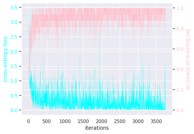
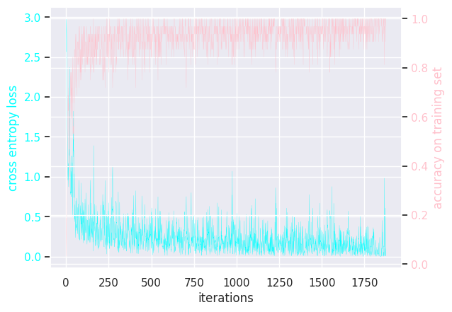
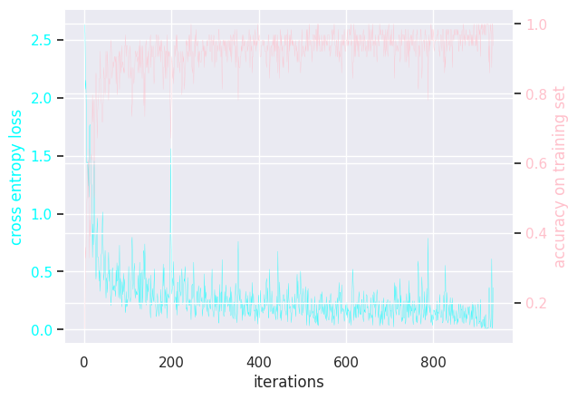
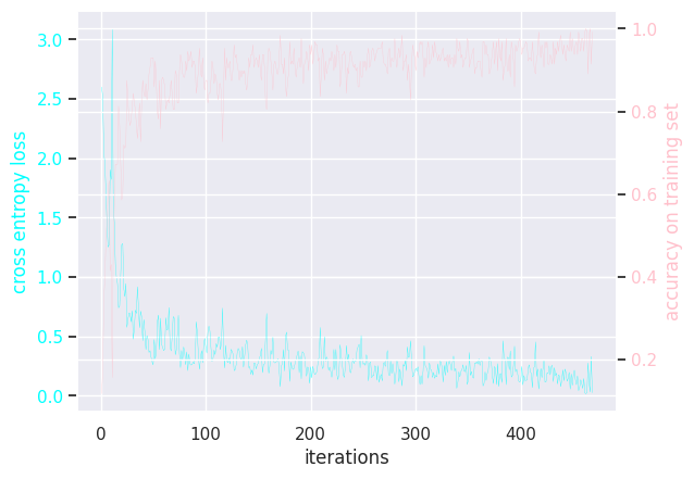
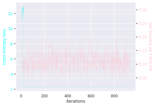
Results of modifying a few hyperparameters:
MLP batch size = 16
MLP batch size = 32
MLP batch size = 64
MLP batch size = 128
MLP learning rate = 0.1
MLP learning rate = 0.01
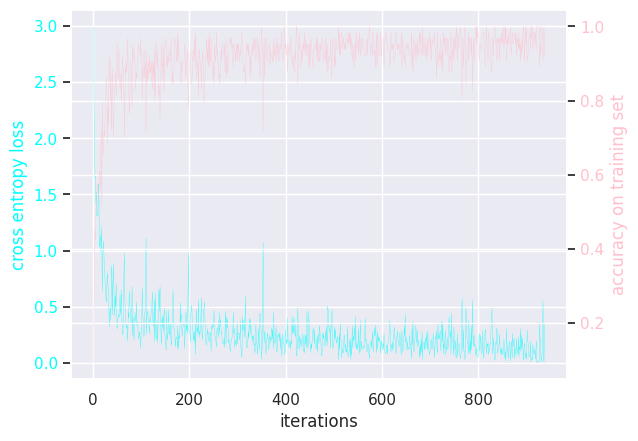
MLP learning rate = 0.001
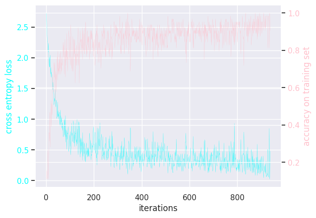
MLP learning rate = 0.0001
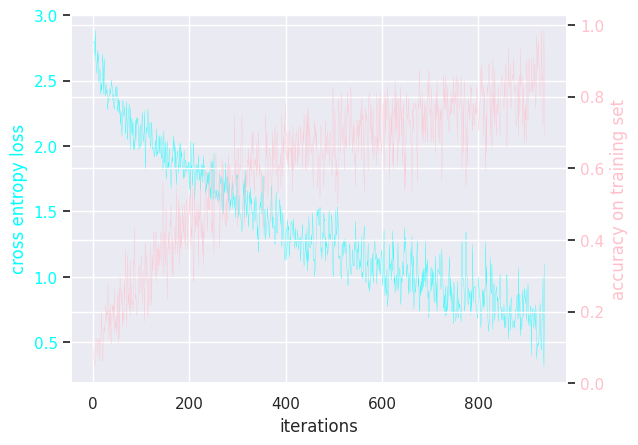
MLP activation relu
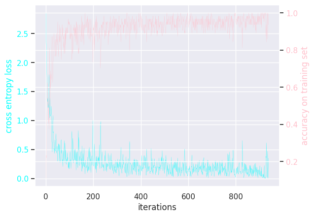
MLP activation sigmoid
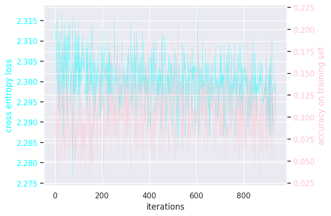
MLP activation tanh
